ch16.Rmd

---
title: "分群模型（Clustering）"
author: "郭耀仁"
date: "`r Sys.Date()`"
output: slidy_presentation
---

```{r setup, include=FALSE}
knitr::opts_chunk$set(echo = TRUE, warning = FALSE, results = 'hide', message = FALSE)
```

## 常見的機器學習問題

- 監督式學習
    - 迴歸模型
    - 分類模型
- 非監督式學習
    - 分群模型（*）

## 分群模型的特性

- 訓練資料集是沒有答案的, 所以沒有對與錯
- 組內差異小
- 組間差異大
- 差異是以觀測值之間的**距離**作為度量

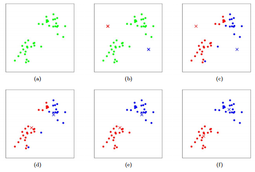
## K-Means

- 隨便放 k 個中心點
- 依照各點與 k 個中心點的距離標記分群
- 然後將中心點移到各群的中心
- 重複上兩個步驟一直到中心點的移動已經收斂
- 如下圖（k = 2）：

![Stanford.edu：K-Means 視覺化](http://stanford.edu/~cpiech/cs221/img/kmeansViz.png)

## `kmeans()` 函數

- 查詢 `kmeans()` 函數
- `centers` 就是 k 值
- `nstart` 是指重新隨意放 k 個中心點的次數, 一般建議 `nstart >= 10`

## `kmeans()` 函數（2）

```{r}
iris_km <- iris[, -5]
set.seed(87)
km_fit <- kmeans(iris_km, nstart = 10, centers = 3)

# Plotting
par(mfrow = c(1, 2))
plot(x = iris$Sepal.Length, y = iris$Sepal.Width, col = iris$Species, main = "Labeled")
plot(x = iris$Sepal.Length, y = iris$Sepal.Width, col = km_fit$cluster, main = "K-Means", ylab = "")
```

## 評估分群模型

- 組內差異（WSS）愈小愈好
- 組間差異（BSS）愈大愈好
- 比例 `Total WSS/Total SS`，這個數值愈低表示績效愈好

```{r}
ratio <- km_fit$tot.withinss / km_fit$totss
ratio
```

## 選擇 k 值

- 隨著 k 增加, `Total WSS/Total SS` 一定會持續下降
- 如果我們讓 k = 觀測值數目, 一定可以得到一個 `Total WSS/Total SS` 最低的結果
- 但這個不會是我們想要的分群方法
- 我們要找的是下降效率開始變小的 k
- 實務上常使用**陡坡圖**來找**手肘點**

## 選擇 k 值（2）

```{r}
ratio_ss <- rep(NA, times = 20)
for (k in 1:length(ratio_ss)) {
  iris_km <- iris[, -5]
  set.seed(87)
  km_fit <- kmeans(iris_km, centers = k, nstart = 10)
  ratio_ss[k] <- km_fit$tot.withinss/km_fit$totss
}
plot(ratio_ss, type = "b", xlab = "k", main = "screeplot")
```

## 標準化

- Standard Scaler
- 使用 `scale()` 函數

```{r}
scaled_iris_mat <- scale(iris[, -5])
scaled_iris_df <- data.frame(scaled_iris_mat)
View(scaled_iris_df)
```

## 標準化（2）

- Min Max Scaler
- 自訂

```{r}
# Self-defined function: min_max_scaler
min_max_scaler <- function(df) {
  col_n <- ncol(df)
  empty_matrix <- matrix(nrow = nrow(df), ncol = ncol(df))
  normalized_df <- data.frame(empty_matrix)
  for (i in 1:col_n) {
    minimum <- min(df[, i])
    maximum <- max(df[, i])
    normalized <- (df[, i] - minimum) / (maximum - minimum)
    normalized_df[, i] <- normalized
  }
  names(normalized_df) <- names(df)
  return(normalized_df)
}

# Function calls
scaled_iris <- min_max_scaler(iris[, -5])
View(scaled_iris)
```